Geophysics and
Electrotechnology
[Geophysics]
Definition: application of physics to studies of the Earth,
Moon, and other planets. It includes Earth, atmosphere, oceans, planetary
systems.
Classification: Pure and applied geophysics, solid Earth, surface
geophysics
Applied geophysics: exploration geophysics, engineering geophysics,
environmental geophysics, groundwater geophysics, archaeo-geophysics, forensics
Exploration geophysics: use of seismic, gravity, magnetic, electrical,
electromagnetic, etc., methods in the search of oil, gas, minerlas, water,
etc., with the objective of economic exploitation.
[Earth's
Structure]
Earth's age: 4.5 by
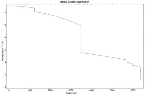
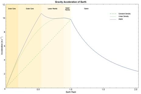
Earth's size: radius 6,400km, circumference 40,000km
Earth's average density: 5.5
Earth's construction:

crust = 30km(locally 5-200km); mantle = to
3000km(upper 30-700km, lower 700-3000km); outer core = 3000-5000km; inner core
= 5000-6400km
[Earth's
Atmosphere]

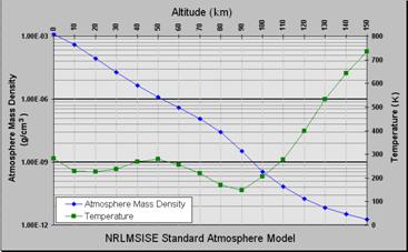
Karman line: 100km above. 99.99997% of the mass of the earth's atmosphere. This marks
the beginning of the space where human travelers are considered astronauts.
Commercial airlines flight height: 10-13km. Thinner aire improves fuel economy.
International Space Station and Space Shuttle: 350-400km. Non-negligible atmospheric drag requires
reboosts every few months.
Ozone layer: 20-30km. high concentration of ozone (O3) created by the
Sun's UV light striking oxygen molecules. Absorbs 97-99% of the Sun's
high-frequency UV light, which potentially damages the life forms on Earth.


[Resistivity
Method, Fundamentals]
Modeling current flow: Current flow is always perpendicular to equipotential lines. Where ground
is uniform, measured resistivity should not change with electrode configuration
and surface location. Where
inhomogeneity present, resistivity varies with electrode position.
Computed value is called apparent resistivity ρA.
Electrode polarization: A metallic electrode like a copper or steel rod in contact with an
electrolyte groundwater other than a saturated solution of one of its own salt
will generate a measurable contact potential. For DC Resistivity, use nonpolarizing
electrodes. Copper and copper sulfate solutions are commonly used.
Elecrtrical anomaly: Different resistivity if measured parallel to the bedding plane compared
to perpendicular to it .
Telluric current: Naturally existing current flow within the earth. By periodically
reversing the current from the current electrodes or by employing a slowly
varying AC current, the affects of
telluric can be cancelled.
Point current source impressed on a half-space:
![]()
![]()

![]()
![]()
Depth of current penetration: Current flow tends to occur close to the surface.
Current penetration can be increased by increasing separation of current
electrodes. Proportion of current flowing beneath depth z as a function of
current electrode separation AB:
Electrode configurations: The value of the apparent resistivity depends on the geometry of the
electrode array used (K factor)
1) Wenner arrangement (1916): The four electrodes A , M , N , B are equally spaced along a
straight line. The distance between adjacent electrode is called “a” spacing . So AM=MN=NB= ⅓ AB = a. This array is
sensitive to horizontal variations.
![]()
2) Lee's partitioning array: This array is the same
as the wenner array, except that an additional potential electrode O is placed
at the center of the array between the Potential electrodes M and N.
Measurements of the potential difference are made between O and M and between O
and N .
![]()
3) Schlumberger arrangement: This array is the most
widely used in the electrical prospecting . Four electrodes are placed along a
straight line in the same order AMNB
, but with AB ≥ 5 MN. This array is less sensitive to
lateral variations and faster to use as only the current electrodes are moved.

4) Dipole-dipole array: The use of the dipole-dipole arrays
has become common since the 1950’s , Particularly in Russia. In a
dipole-dipole, the distance between the current electrode A and B (current dipole)
and the distance between the potential electrodes M and N (measuring
dipole) are significantly smaller than the distance r , between the centers of the two dipoles. This array is used for
deep penetration ≈ 1 km
![]()
Azimuthal, radial, parallel and perpendicular
arrangements are four basic configurations of the dipole array. When the
azimuth angle (θ) formed by the line r and the current dipole AB is π /2 , the azimuthal array
and parallel array reduce to the equatorial array. When θ= 0 , the
parallel and radial arrays reduce to the polar or axial array. If MN only is small is small with respect
to r in the equatorial array, the
system is called bipole-dipole (AB is
the bipole and MN is the dipole ),
where AB is large and MN is small. If AB and MN are both small with respect to r, the system is dipole- dipole.
5) Pole-dipole array: The second current electrode
is assumed to be a great distance from the measurement location (infinite
electrode).
![]()
6) Pole-pole array: If one of the potential
electrodes , N is also at a great distance.
![]()
Material boundaries:
1) Refraction : the current flow is refracted on a
material boundary.
![]()
![]() (P in medium 1)
(P in medium 1)
![]() (reflection
coefficient)
(reflection
coefficient)
![]() (P in medium 2)
(P in medium 2)
![]()
2) Method of images: Two media separated by semi
transparent mirror of reflection and transmission coefficients k and 1-k, with light source in medium 1. Intensity at a point in medium 1
is due to source and its reflection, considered as image source in second
medium, i.e source scaled by reflection coefficient k. Intensity at point in medium 2 is due only to source scaled by
transmission coefficient 1-k as light
passed through boundary.
Vertical electrical sounding (VES): The object of
VES is to deduce the variation of resistivity with depth below a given point on
the ground surface and to correlate it with the available geological
information in order to infer the depths and resistivities of the layers
present. In VES, with wenner configuration, the array spacing “a” is increased by steps, keeping the
midpoint fixed (a = 2 , 6, 18,
54…….). In VES, with schlumberger, The potential electrodes are moved only
occasionally, and current electrode are systematically moved outwards in steps AB > 5MN.
Horizontal electrical profiling (HEP): The object of
HEP is to detect lateral variations in the resistivity of the ground, such as
lithological changes, near- surface faults. In the wenner procedurec
of HEP , the four electrodes with a definite array spacing “a” is moved as a whole in suitable
steps, say 10-20 m. four electrodes are moving after each measurement. In the
schlumberger method of HEP, the current electrodes remain fixed at a relatively
large distance, for instance, a few hundred meters , and the potential
electrode with a small constant separation (MN)
are moved between A and B.
Three-layer structure: For Three layers
resistivities in two interface case , four possible curve types exist.
Q- type : ρ1 > ρ2 > ρ3, H-type: ρ1 > ρ2 < ρ3, K-type: ρ1 < ρ2 > ρ3, A-type: ρ1 < ρ2 < ρ3.
Four-layer
structure: 8 possible relations. HA, HK,
AA, AK, KH, KQ, QH, QQ types
Quantitative VES interpretation: Layer
resistivity values can be estimated by matching to a set of master curves
calculated assuming a layered Earth, in which layer thickness increases with
depth. (seems to work well). For two layers, master curves can be represented
on a single plot. Master curves: log-log plot with ρA
/ ρ1 on vertical axis and a / h
on horizontal (h is depth to
interface).
Plot smoothed
field data on log-log graph transparency. Overlay transparency on master curves
keeping axes parallel. Note electrode spacing on transparency at which (a / h=1)
to get interface depth. Note electrode spacing on transparency at which (ρA / ρ1 =1) to get resistivity of layer 1. Read off value of k to calculate resistivity of layer 2
from.
Curve matching
is also used for three layer models, but book of many more curves. Recently,
computer-based methods have become common: forward modeling with layer
thicknesses and resistivities provided by user, inversion methods where model
parameters iteratively estimated from data subject to user supplied constraints
Example
(Barker, 1992): Start with model of as many layers as data points and resistivity
equal to measured apparent resistivity value.
Calculated
curve does not match data, but can be perturbed to improve fit.
Principle
of equivalence: If we consider three-lager curves of K (ρ1 < ρ2 > ρ3 ) or Q
type (ρ1 > ρ2 > ρ3) we find the
possible range of values for the product T2= ρ2 h2 turns out to be much
smaller. This is called T-equivalence. H = thickness, T: transverse
resistance it implies that we can determine T2
more reliably than ρ2 and h2 separately. If we can
estimate either ρ2 or h2 independently we can
narrow the ambiguity. Equivalence: several models produce the same results.
Ambiguity in physics of 1D interpretation such that different layered models
basically yield the same response.
Different
Scenarios: conductive layers between two resistors, where lateral conductance (σh) is the same. Resistive layer between
two conductors with same transverse resistance (ρh).
Principle
of suppression: a thin layer may sometimes not be detectable on the
field graph within the errors of field measurements. The thin layer will then
be averaged into on overlying or underlying layer in the interpretation. Thin
layers of small resistivity contrast with respect to background will be missed.
Thin layers of greater resistivity contrast will be detectable, but equivalence
limits resolution of boundary depths, etc.
The
detectibility of a layer of given resistivity depends on its relative thickness
which is defined as the ratio of thickness/depth.
Advantages
of resistivity method: flexible, relatively rapid. field time increases
with depth, minimal field expenses other than personnel, Equipment is light and
portable. Qualitative interpretation is straightforward
Respond to
different material properties than do seismic and other methods, specifically
to the water content and water salinity.
Disadvantages
of resistivity method: interpretations are ambiguous, consequently,
independent geophysical and geological controls are necessary to discriminate between
valid alternative interpretation of the resistivity data (principles of suppression
& equivalence). Interpretation is limited to simple structural
configurations. Topography and the effects of near surface resistivity
variations can mask the effects of deeper variations. The depth of penetration
of the method is limited by the maximum electrical power that can be introduced
into the ground and by the practical difficulties of laying out long length of
cable. The practical depth limit of most surveys is about 1km. Accuracy of
depth determination is substantially lower than with seismic methods or with drilling.
[Mise-A-La-Masse Method]
This is a
charged-body potential method is a development of HEP technique but involves
placing one current electrode within a conducting body and the other current
electrode at a semi- infinite distance away on the surface. This method is
useful in checking whether a particular conductive mineral- show forms an
isolated mass or is part of a larger electrically connected ore body.
[Self-Potential
(SP) Method]
SP is called
also spontaneous polarization and is a naturally occurring potential difference
between points in the ground. SP depends on small potentials or voltages being
naturally produced by some massive ores. It associate with sulphide and some
other types of ores. It works strongly on pyrite, pyrrohotite, chalcopyrite,
graphite. SP is the cheapest of geophysical methods.
Conditions for
SP anomalies: shallow ore body. Continuous extension from a zone of oxidizing
conditions to one of reducing conditions, such as above and below water table.
Electrochemical
mechanism of SP: The ore body must be an electronic conductor with
high conductivity. This would seem to eliminate sphalerite (zinc sulfide) which
has low conductivity. The ore body must be electrically continuous between a
region of oxidizing conditions and a region of reducing conditions. While water
table contact would not be the only possibility have, it would seem to be a
favorable one. Mineral potential (ores that conduct electronically ) such as
most sulphide ores, not sphalerite (zinc sulphide) magnetite, graphite. Potential
anomaly over sulfide or graphite body is negative The ore body being a good
conductor. Curries current from oxidizing electrolytes above water - table to
reducing one below it .
Diffusion
potential:
![]()
Ia, Ic
: mobilities of the anions (+ve) and cations (-ve)
R : universal gas constant (8.314 J K-1 mol-1)
T : absolute temperature (K)
n : ionic valence
F : Faraday's constant (96487 C mol-1)
C1, C2
: solution concentration
Nernst
potential:
![]()
Instrumentation
for SP: Since we wish to detect currents, a natural approach is to measure
current. However, the process of measurement alters the current. Therefore, we
arrive at it though measuring potentials.
potentiometer
or high impedance voltmeter, 2 non-polarizing electrodes, wire and reel. Non-polarizing
electrodes were described in connection with resistivity exploration although
they are not usually required there. Here, they are essential. The use of
simple metal electrodes would generate huge contact or corrosion potentials
which would mask the desired effect. non-polarizing electrodes consist of a
metal in contact with a saturated solution of a salt of the metal. Contact
with the earth can be made through a porous ceramic pot.
The instrument
which measures potential difference between the electrodes must have the
following characteristics: capable of measuring +0.1 millivolt, capable of
measuring up to ±1000 millivolts (±1 volt)
input
impedance greater than 10 megaohms, preferably more. The high input impedance
is required in order to avoid drawing current through the electrodes, whose
resistance is usually less than 100 kilohms. In very dry conditions (dry rock,
ice, snow, frozen soil), the electrode resistance may exceed 100 kilohms, in
which case the instrument input impedance should also be increased.
SP
Interpretation: Usually, interpretation consists of looking for
anomalies. The order of magnitude of anomalies is 0-20 mv normal variation, 20-50
mv possibly of interest, especially if observed over a fairly large area, over
50 mv definite anomaly, 400-1000 mv very large anomalies.
[Induced
Polarization (IP) Method]
IP depends on
a small amount of electric charge being stored in an ore when a current is
passed through it , to be released and measured when the current is switched off.
The main application is in the search for disseminated metallic ores and to a
lesser extent, ground water and geothermal exploration. Measurements of IP
using 2 current electrodes and 2 non-polarizable potential electrodes. When the
current is switched off , the voltage between the potential electrodes takes a
finite to decay to zero because the ground temporarily stores charge (become polarized).
IP is A bulk
effect. Grain (electrode) polarization. (A) Unrestricted electrolytic flow in
an open channel.
(B) Polarization
of an electronically conductive grain, blocking a channel.
Types of IP
instrumentation: time domain, frequency domain (< 10Hz), phase domain,
spectral IP (10-3 - 4000Hz)
Time-domain
measurement: One measure of the IP effects is the ratio Vp / Vo
which is known chargeability which expressed in terms of millivolts per volt or
percent. i : overvoltage
Vo : observed
voltage
Inonosphere: 85-600km. Atmospheric gases are ionized
by solar radiation (mostly UV)


D layer: 60-90km.
HF waves ( < 10MHz) are not reflected but attenuated. Disappearance of the D
layer is reponsible for the reception of distant AM broadcast at night times.
E layer: 90-120km. At oblique incidence, HF waves (
< 10MHz) are reflected by E layer.
F layer: 200-500km. Highest ionization density.
Responsible for skywave radio propagation.
Ionospheric model: A mathematical description of the
ionosphere (location, altitude, day of year, phase of the sunspot cycle,
geomagnetic activity). The state of the ionospheric plasma may be described by
four parameters: electron density, electron temperature, ion temperature, and
ionic concetration. Radio propagation depends uniquely on electron density.
Most widely used model is the IRI 2007. IRI (International Reference Ionopsher)
Ionograms: Ionograms show the virtual heights and critical frequencies of the ionospheric layers and which are
measured by an ionosonde. An
ionosonde sweeps a range of frequencies, usually from 0.1 to 30 MHz,
transmitting at vertical incidence to the ionosphere. As the frequency
increases, each wave is refracted less by the ionization in the layer, and so
each penetrates further before it is reflected. Eventually, a frequency is
reached that enables the wave to penetrate the layer without being reflected.
For ordinary mode waves, this occurs when the transmitted frequency just
exceeds the peak plasma, or critical, frequency of the layer. Tracings of the
reflected high frequency radio pulses are known as ionograms.
Radiowave interaction with
ionosphere: the incident electric
field forces the electrons into oscillation
at the same frequency as the radio wave. Some of the radio-frequency energy is
given up to this resonant oscillation. The oscillating electrons will then
either be lost to recombination or will re-radiate the original wave energy.
Total refraction can occur when the collision frequency of the ionosphere is
less than the radio frequency, and if the electron density in the ionosphere is
great enough.
The critical frequency is the limiting frequency at
or below which a radio wave is reflected by an ionospheric layer at vertical incidence. If the transmitted frequency is
higher than the plasma frequency of the ionosphere, then the
electrons cannot respond fast enough, and they are not able to re-radiate the
signal.
![]() (critical
frequency in MHz)
(critical
frequency in MHz)
N : electron density per cm3
![]() (maximum usable
frquency)
(maximum usable
frquency)
α : angle of attack relative to the
horizon
DX communication: Employs the ionospheric reflection of the radio wave up
to 5 hops. DX communication is the hobby of receiving and identifying distant radio
or television
signals, or making two way radio contact with distant stations in amateur radio, citizens' band
radio or other two way radio communications. It is usually done in
AM, shortwave and VHF bands.
Incoherent scatter radar: Probes the ionosphere above the critical frequencies.
The power spectrum contains information not only on the density, but also on
the ion and electron temperatures, ion masses and drift velocities. EISCAT,
Sondre Stromfjord, Milstone Hill, Arecibo, and Jicamara radars.
Coherent backscatter radar: 8-20MHz. similar to Bragg scattering in crystals and
involves the constructive interference of scattering from ionospheric density
irregularities. SuperDARN radar project.
HARRP (High Frequency Active Auroal Research Program):
high power radio transmitters to modify the properties of the ionosphere. to
enhance communications and surveillance systems for both civilian and military
purposes. HAARP was started in 1993 as a proposed twenty year experiment, and
is currently active near Gakona, Alaska.
[Geophysical
Methods]
Overview: critical to select correct tool(s) for objective
either alone or part of a larger survey
Gravity method:
Magnetic mehod:
Seismic method: reflection, refraction, surface or borehole
Ground penetrating radar method:
Resistivity method:
Frequency = DC or
slowyly-varying AC source
Principles = measure resitance between two electrodes submerged into the Earth at a
certain depth. The presence of pore fluids and clays affect the resistance. The
apparent resistivity is a function of the measured resistance and the geometry
of the electrode array. In the shallow subsurface, the presence of water
controls much of the conductivity variation. Mesurement of resistivity is, in
general, a measure of water saturation and connectivity of pore space.
Increasing saturation, increasing salinity of the underground water, increasing
porosity of rock (water-filled voids) and increasing number of fractures
(water-filled) all tend to decrease measured resistivity. Increasing compaction
of soils or rock units will expel water and effectively increase resistivity.
Resisity of common geological materials (ohm-m), typical values = Ignenous rocks 104, metamorphic rocks
103, sedimentary rocks 103, unconsolidated 103,
ground water 5, pure water 103
Current flow by electron movements: in metals. Metals may be considered a special class
of electron semiconductor for which E
approaches zero. Most sulfide ore minerals are electron semiconductors with
small E.
Current flow by ion movements: in salt water. Most earth materials conduct
electricity by the motion of ions contained in the water with the pore spaces.
Electric polarization: ions or electrons move only a short distance (under an electric field)
and then stop
Good electrical contanct with the earth: wet
electrode location, add NaCl solution or bentonite
Induced polarization
method: done in
conjuction with DC resistivity. It measures the transient (short-term)
variations in potential as the current is initially applied or removed from the
ground. The ground behaves much like a capacitor, storing some of the applied
current as a charge that is dissipated upon removal of the current. Both
capacity and electrochemical effects are responsible. IP is commonly used to
detect concentrations of clay and electrically conductive metallic mineral
grains.
Self potential (SP)
method: passive
method of measuring the naturally occuring electrical potentials commonly
associated with the weathering of sulfide ore bodies. Electric potential can be
also observed in association with ground-water flow and certain biologic
processes. A high-impedance voltmeter and some means of making good electrical
contact to the ground are required.
Electromagnetic (EM)
method: a
time-varying magnetic field is generated at the surface of the earth, which in
turn produces a time-varying electric current in the earth through induction. A
receiver compares the magentic field due to the induced current to that
generated by the source. It is used for locating conductive base-metal
deposits, buried pipes and cables, unexploded ordinance, and for near-surface
geophysical mapping.
Magnetotelluric (MT)
method: a
passive method that measures naturally occuring electrical currents, telluric
currents, generated by magnetic induction of electric currents in the
ionosphere. Used to determine electrical properties of materials at relatively
great depths (down to and including the mantle) inside the Earth. A time
variation of electric potential is measured at a base station and at survey
stations. Differences in the recorded signal are used to estimate subsurface
distribution of electrical resistivity.
EM method:
Borehole survey:
[Technical
Issues in Geophysics]
Spatical aliasing:
Survey noise: types of survey noise
Elimination of survey noise: data
processing for noise elimination, coherent integration
Data display: 1D profile, 2D colour on a plane, 2D gray photo
(topographic) such as a SAR image, 3D grid
[Electrotechnology
in Volcanic Monitoring]
Electric methods:
changes in
electrical resistivity in advance of eruptions and during magmatic intrusion
events. Resistivity structure to a depth of 5km beneath a volcano from
large-loop-source electromagnetic measurements (0.04-8Hz)
Magnetic methods: magnetotelluric(MT) sounding, estimation of
sub-surface temperature, deep temperature extrapolation, 3D interpretation of
MT data in volcanic environments
Electromagnetic
methods: electromagnetic induction. 3D temperature model from
electromagnetic data, temperature extropolation in depth by an indirect
electromagnetic geothermometer, electromagnetic sounding of the Earth's
interior, construction of 3D geoelectric models from electromagnetic data,
solving external boundary value problems in geoelectromagnetism
Self-potential methods: measure transient changes in the self-potential
field associated with changes in hydro
thermal circulation due to volcanic activity
Satellite-based
electrotchnologies:
[Websites]
Virtual ElectroMagnetic Laboratory (VEML), Inst. of
the Russian Academy of Sciences, Geophysical Center of RAS: http://virtual-electromagnetic-laboratory.com/index.html
[References]
B. Singh, Ed., Electromagnetic
Phenomenon Related to Earthquakes and Volcanoes, Narosa,
G. Lavecchia and G. Scalera, Eds., Magneti, Electric and Electromagnetic
Methods in Seismology and
Volcanology, Proc. IV Int. Workshop, La Londe Les Maures,
France, Sept. 5-9, 2004.
Anals of Geophysics
Electromagnetic Sounding of the Earth's Interior,
Elsevier,
B. Spies and M. Oristaglio, 3-D Electromagnetics, SEG Publications, GD7, Tulsa