Electromagnetics
01, Python Coding
1.
파이썬 온라인 자습서
ㅇ Tutorials Point 'Learn Python': https://www.tutorialspoint.com/python/index.htm
2.
오픈소스 파이썬 코딩툴 Online
Python 사용법
ㅇ
https://www.online-python.com/
에 접속하여 소스코드를 위창에 copy
ㅇ [Run]아이콘 클릭
ㅇ
아래 창에 데이터
입력 prompt가
표시되면 키보드로 데이터
입력한다. 출력은
같은 창에 표시된다.
ㅇ
결과를 문서(보고서)에 붙여
넣기
-
하단창 상단의 [Stop] 아이콘 클릭
-
하단창 좌측 첫번째
아이콘 ![]() 클릭하여 결과 텍스트를 Clipboard에 삽입
클릭하여 결과 텍스트를 Clipboard에 삽입
- 결과를 삽입하려는 문서로 이동하여 삽입위치에 커서를 위치 시킨다.
- 키보드에서 Ctrl + V를 누르면 결과 텍스트가 다음과 같이 문서에 삽입된다.
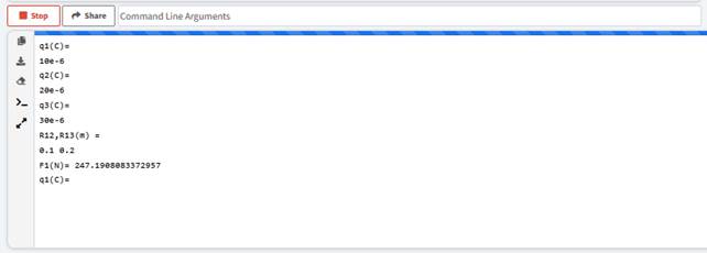
q1(C)=
10e-6
q2(C)=
20e-6
q3(C)=
30e-6
R12,R13(m)
=
0.1
0.2
F1(N)=
247.1908083372957
q1(C)=
Session
Killed due to Timeout.
Press
Enter to exit terminal
(참고)
ㅇ
상단창(소스코드창) 상단에 배치된 아이콘
메뉴 의미
상단좌측
아이콘 4개: Open file From Disk, Save File to
Disk, Undo, Redo
상단우측
아이콘 3개: Change Theme, About Site,
Settings
ㅇ
하단창(입출력창) 좌측 아이콘 메뉴 5개의 의미
Copy
to clipboard: 출력창 내용을 클립보드에 copy (다음에 Ctrl+v로
문서에 삽입)
Download:
출력창 내용을 txt 파일로 컴퓨터로 다운로드
Clear:
출력창 내용 지움
Smart
terminal: >>>가 표시되고 interpreter 모드. Python를 1줄씩 실행. help(print)
와 같이 help 표시
Expand/Collapse:
Expand = 출력창만 전체화면에 표시, Collapse: 위창, 아래창 동시표시
3. 파이썬 코딩실습
3.1 Example 1: 쿨롱의 법칙
1) 문제
Medium:
air, ε0 = 8.854×10⁻¹²
F/m
q1
= 10 μC, q2 = 20 μC, q2 = 30 μC
q1
at (x, y, z) = (10, 0, 0) cm
q2
at (20, 0, 0) cm
q3
at (30, 0, 0) cm
Find
the electrostatic force magnitude F1
on q1.
(Solution)
2) 수식
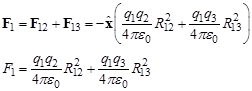
q in C (coulomb)
R in m (meter)
ε0 in F/m (farad per meter)
F in N (newton)
q1
= 10 μC = 10e-6 C
q2
= 20 μC = 20e-6 C
q3
= 30 μC = 30e-6 C
R12
= 20 - 10 = 10 cm = 0.1 m
R13
= 30 - 10 = 20 cm = 0.2 m
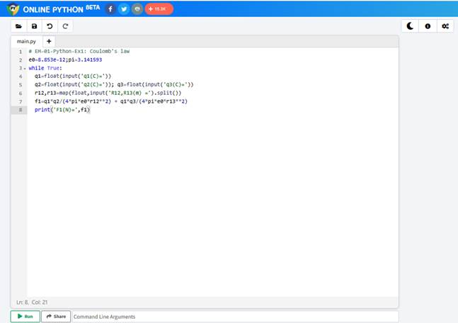
3) 코딩
# EM-01-Python-Ex1: Coulomb's law
e0=8.853e-12;pi=3.141593
while True: # 무한루프.
프로그램을 중지시키기 전까지 계속 수행
q1=float(input('q1(C)=')) # while 블록
소속된 프로그램
줄은 동일
칸만큼 들여쓰기
q2=float(input('q2(C)=')); q3=float(input('q3(C)=')) #여러
줄 프로그램
줄을 ; 사용하여 한
줄에
# 키보드로 입력되는 모든 문자는 character로 취급.
float을 사용하여
실수형 변환
r12,r13=map(float,input('R12,R13(m) =').split()) #2개 데이터 한줄에 입력. 사이에 space
f1=q1*q2/(4*pi*e0*r12**2) + q1*q3/(4*pi*e0*r13**2)
print('F1(N)=',f1)
(참고) Python에서 comment
#
This is a comment.
y=2*x+3
# A linear function
"""
This
is a multi-line comment.
Comment
starts.
Comment
ends.
"""
'''
This
is a multi-line comment.
Comment
starts.
Comment
ends.
'''
여러줄 comment: 큰 인용부(") 또는 작은 인용부(') 3개로 둘러 싸인
부분
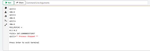
4) 코드 수행결과
q1(C)=
10e-6
q2(C)=
20e-6
q3(C)=
30e-6
R12,R13(m)
=
0.1
0.2
F1(N)=
247.1908083372957
q1(C)=**
Process Stopped **
Press
Enter to exit terminal
3.2 Example 2: 무한 선전류의 자기장 계산
1) 문제
Medium:
air, μ0 = 8.854×10⁻¹²
H/m
I = 1000 A (756 kV 초고압 송전선)
r = 30 m (송전선과
지면 사이 거리)
Find
the magnetic flux density B (G)
B in G (gauss), 1 G = 0.1 mT = 10-4 T, T (Tesla)
2) 수식
![]()
I in A
μ0 in H/m
r in m
B in T
3) 코딩
#
EM-01-Python-Ex2: Magnetic field of a line current
pi=3.141593;
u0=4*pi*1e-7
while
True:
I=float(input('I(A)='))
r=float(input('r(m)='))
B=u0*I/(4*pi*r)*1e4
print('B(G)=',B)
4) 코드 수행결과
I(A)=
1000
r(m)=
30
B(G)=
0.033333333333333326
I(A)=**
Process Stopped **
Press
Enter to exit terminal
3.3 Example 3:
(참고) Python에서 복소수 연산
(Complex
numbers in Python)
ㅇ 표기: 1+2j, 1.+1.j, 2j
ㅇ 입력시 괄호 없이 1+2j와 같이 입력
ㅇ 출력시 괄호가 사용됨 (실수, 허수 모두 있을 때)
2j
(1+2j)
ㅇ 실수부와 허수부는 실수 규칙을 따름.
ㅇ 복소수 지정
z=3+2j
z=complex(3,2)
ㅇ 복소수 연산
4칙연산: + - * / **
z1+z2, z1-z2, z1*z2, z1/z2
z1**2, pow(z, 2), z1**z2
z.real
z.imag
z.conjugate()
z=complex(x, y)
z=complex(2, 4)
z=complex(2) # z=2+0j
ㅇ 복소수 라이브러리 함수
from cmath import *
exp(z), phase(z), abs(z),
polar(z),rect(r, phi), log(z, [base]), log10(z), sqrt(z)
acos(z), asin(z), atan(z), cos(z),
sin(z), tan(z)
acosh(z), asinh(z), atanh(z),
cosh(z), sinh(z), tanh(z)
1) 문제
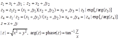
복소수 z1과 z2를 입력받아 z3 = z1*z2, z4=z1/z2를 실수/허수, 크기/위상(radian)으로 표시
2) 수식
3) 코딩
# EM-01-Python-Ex3: Complex
calulation
from cmath import * # Use the complex
math library in Python
while True:
z1=complex(input('z1='))
z2=complex(input('z2='))
z3=z1*z2; z4=z1/z2
zp3=polar(z3); zp4=polar(z4)
print('z3=',z3,'z3(polar)=',zp3)
print('z4=',z4, 'z4(polar)=',zp4)
4) 코드 수행결과
z1=
1+2j
z2=
3+4j
z3= (-5+10j) z3(polar)=
(11.180339887498949, 2.0344439357957027)
z4= (0.44+0.08j) z4(polar)=
(0.4472135954999579, 0.17985349979247828)
z1=** Process Stopped **
Press Enter to exit terminal
3.4 Example 4: R, L, C
serie circuit impedance
1) 문제
R, L, C, f 가 주어진 경우 RLC 직렬회로와 RLC 병렬회로의 임피던스를 계산하라.
2) 수식
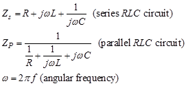
R in Ω (Ohm)
L in H (Henry)
C in F (Farad)
ω in rad/s
f in Hz (Herz)
3) 코딩
#
EM-01-Python-Ex4: RLC series and parallel circuits
pi=3.141593
while
True:
R=float(input('R(ohm)='))
L=float(input('L(uH)='))
C=float(input('C(uF)='))
f=float(input('f(Hz)='))
w=2*pi*f
Zs=complex(R, w*L*1e-6-1/(w*C*1e-6))
Zp=1/complex(1/R, w*C*1e-6-1/(w*L*1e-6))
print('Z(series)=', Zs)
print('Z(parallel)=', Zp)
4) 코드 수행결과
R(ohm)=
100
L(uH)=
20
C(uF)=
50
f(Hz)=
1e6
Z(series)=
(100+125.66053690148915j)
Z(parallel)=
(1.0132629437904996e-07-0.0031831791384774404j)
R(ohm)=**
Process Stopped **
Press
Enter to exit terminal