ICT083 Antenna Design

Reflector Antennas

I. Theory

1. Optics-based Antennas

- Reflector antennas

- Lens antennas

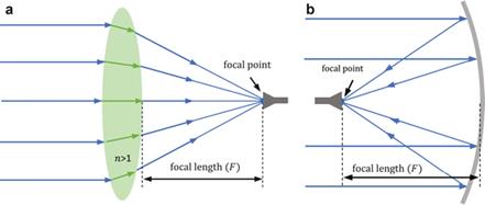
Figure: Optical antennas. Left = lens antenna, right = parabolic reflector antenna [C. A. Fernandes et al. in Handbook of Antenna Technologies, Z. N. Chen et al. Ed. Springer, 2016]

Figure: A geometrical optics ray tracing for the upgraded (1997) Arecibo radiotelescope [Hecht, Optics, Fourth Edition]

2. Reflector Antenna Types

Figure: Reflector antennas in various forms [Hazdra (2015)]

- Feed

A small antenna illuminating the reflector. Waveguide radiators and horns are most widely used.

- Signle reflector

Reflector's surface is a parabolid.

Prime-focus reflector: Feed at the reflector's frontal center.

Offset reflector: Part of the parabolic surface is used.

- Dual-reflector antenna

Main reflector + subreflector

Cassegrain reflector: Paraboloidal surface + hyperboloidal surface

Gregorian reflector: Paraboloidal surface + ellipsoidal surface

Figure: A Cassegrain reflectgor antenna fed by a four-reflector beam waveguide [Chiba (2011)] and a multibeam antenna in an offset single reflector configuration [Greda (2010)].

- Beam-waveguide fed reflector antenna: Feed's pattern is routed to a subreflector via a wave beam. For large reflectors. The transceiver can be located inside an instrument room.

- Multi-beam reflector antenna antenna: Has multiple beams with multiple input/output ports. Uses an array feed. Used in satellite communications.

3. Wave-front Transforming Surface in Reflector Antennas

- The three most important surfaces in reflector antenna design are parabolidal, ellipsoidal, and hyperboloidal surfaces.

Figure: Reflector surfaces useful in antenna engineering [Bely, The Design and Construction of Large Optical Telescopes].

1) Paraboloidal Surface

- Transforma a spherical wave into a planewave.

- Feed's aperture area is greatly increased by the reflecting surface.

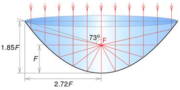
Figure: A paraboloidal reflector [Wikipedia].

2) Ellipsoidal Surface

- Transforma a spherical wave into a spherical wave.

- The primay focal point (of the main refector) is moved toward the main reflector

- The secondary focal point (of the subreflector) is located between the subreflector and the main reflector.

Figure: Ray reflections on ellipsoidal and hyperboloidal surfaces [Bely, The Design and Construction of Large Optical Telescopes].

3) Hyperboloidal Surface

- Transforma a spherical wave into a spherical wave.

- The primay focal point (of the main refector) is moved toward the main reflector

- The secondary focal point (of the subreflector) is located behind the subreflector away from the main reflector.

4) Spheroidal Surface

- Focal points are distributed along the symmetry axis. Thus a line source is used.

- The linear distribution of focal points can be made to converge to a single point by using a shaped subreflector.

Figure: Ray tracking on a pheroidal reflecting surface [Physics LibreTexts]. Focal points can be made to converge to a point by using a shaped subreflector [Monk (2001)].

- Spherodial surface is very useful in multi-beam and wide-angle scanning applications.

Figure: Multibeam property of a spheroidal reflecting surface [Jiang (2019)].

4. Parabolic Reflector Antenna

- The most important form of a reflector antenna

- Theory of operation: conversion of a spherical wave into a planewave

- Ray path length independent of the ray angle

Figure: Geometry of a parabolic reflector [Hazdra (2015)].

- Various types of the reflector antenna

- Origin at the reflector apex

- F-A-A' path length = F-B-B' path length

Figure: Trasformation of a spherical wavefront into a planar wavefront by a parabolidal reflector.

- Origin at the focal point

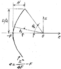
Figure: Parabolic reflector geometry with an origin at the reflector's apex.

- Space taper

- Feed-oriented geometrical equations

Figure: Parabolic reflector geometry with an origin at the reflector's focus.

3. Parabolic Reflector Antenna Design Procedures

- Maximum efficiecny condition

Figure: Feed illumination loss and spillover loss [Wade].

Figure: Optimum edge taper in the reflector illumination [Hazdra (2015)].

- Feed taper due to spherical wave spreading

Figure: Spherical wave spreading loss [Hazdra (2015)].

Figure: Simulation of a parabolic reflector antenna [Hazdra (2015)].

- Gain speficied

- Calculate the reflector diameter assuming 50% efficiency (when realized).

- Design a feed and find its 10-dB half-beamwidth .

- Design a parabolic reflector.

z: axial distance from the apex

x: radial distance from the apex

- Simulate the reflector illuminated by the feed.

Full-wave simulation

Full-wave symmetrical simmulation: 1/2, 1/4 of the structure applying the field symmetry

Simulation using the far field of the feed

- Analyze the reflector performance.

Figure: 3D gain patterns of a 15-wavelength parabolic reflector [Hazdra (2015)].

- Co-pol. pattern: Large sidelobes (due to reflector rim diffraction) in principal planes (φ = 0° and φ = 90°) at around θ = 90°.

- Cross-pol. pattern: Gain is largest on diagonal planes (φ = 45° and φ = -45°). Strong back radation.

Figure: Cartesian gain patterns of a 15-wavelength refelctor antenna [Hazdra (2015)].

- Reflector's gain pattern standard form:

Co-pol. pattern cuts in principal planes (φ = 0° and φ = 90°)

Cross-pol. pattern cuts in the diagonal plane (φ = 45°)

Pattern angle θ from -180° to +180° to analyze close-in and far-out sidelobes and the fron-to-back ratio.

5. Feed Design

1) Feed Requirements

- Meet a specified 10-dB half beamwidth: 60-80° for prime-focus reflectors and 20-30° for dual reflectors.

- E- and H-plane pattern symmetry

- Low cross polarization

- Good impedance matching: |S11| < -17 dB to account for increase in reflection coeffcient due to reflections at subreflector or main reflector surface.

- Small back radiation.

- Small cross section for reduced aperture blockage and scattering by the feed

- Phase center stability with frequency

2) Reflector Antenna's Pattern Performance

- Sidelobe level:

A uniform circular aperture: SLL = -17.6 dB

A uniform rectangular aperture: SLL = -13.3 dB

- Directivity:

: uniform circular aperture

a : aperture radius

: uniform rectangular aperture

a, b: aperture width and height

- Half-power beamwidth:

: uniform circular aperture

: uniform rectangular aperture

- Sidelobe reduction: Use a tapered aperture. Power density is larger at the aperture center.

16-dB edge taper: -24 dB SLL

Figure: Performance of tapered circular apertuers [W. L. Stutzman].

3) Feed Types

- 18-25 dB gain horns for the Cassegrain reflector

- 8-12 dB gain circular waveguides for the prime-focus parabolic reflector

4) Feed Pattern Analysis

- Reflection coefficient

- 10-dB beamwidth

- E- and H-plane pattern symmetry

- Cross polarization level

- Phase center

- An example: A circular waveguide feed [Koala (2017)]

Aperture diameter 20.53 mm, feed length 60 mm, wall thickness 1 mm

Phase center: At the center of the aperture

Figure: A circular waveguide feed geometry.

Figure: A circular waveguide feed's reflection coefficient.

Figure: Gain and phase patterns of a circular waveguide feed.

5) Cicular Waveguide Feed

- Good E- and H-plane pattern symmetry when the waveguide diameter is 0.65 wavelength.

- Backlobe supperssion: Use a quarter-wave choke around the aperture

- E-plane slits (two of them): To improve the pattern symmetry

5. Reflector Antenna Theoretical Analysis

5.1 Radiation pattern calculation

1) 1D Aperture Integration

- Axi-symmetric case:

: reflector's pattern angle

: feed's pattern angle

- Calculation of Bessel function J₀(x):

Single-precision Fortran

Modification of Abramowitz & Stegun for 0.001 accuracy

2) 2D Aperture Integration

- Use the FFT algorithm with zero-padding

3) Feed Blockage and Scattering Modeling

- Analytically subtract the radiation by the blockage area.

- Feed scattering modeling: Use full-wave simulation.

4) High-frequency Methods

- PO

- Ray methods: GTD, PTD, UTD

- Effects of the aperture blockage

Efficiency decrease due physical blockage: simple formula available

Sidelobe increase: simple formula available

Feed diffraction/scattering efficiency loss: graph available

- Main reflector rim diffraction

Backlobe increase at 180°: main reflector rim diffractions add in phase.

Reduction of rim diffraction:

Rim edge: rolled, castellated, serrated

5.2 Efficiency Calculation

- Maximum directivity

: maximum possible directivity

A_p : antenna aperture's physical area

- Realized directivity

: aperture efficiency

: antenna aperture efficiency

: feed blockage efficiency

: feed diffraction efficiency

: feed amplitude taper efficiency

: feed phase efficiency

: feed spill-over efficiency

: feed cross-polarization efficiency

: implementation efficiecy. Main reflector surface error, feed dielectric loss, feede reflection loss

- Feed lockage efficiency:

- Amplitude taper efficiency:

- Phase error efficiency:

- Spill-over efficiency:

- Cross-polarization efficiency:

- Feed mismatch or reflection efficiency

- Feed material loss efficiency

P_r : power radiated by the antenna

P_t : power transferred to the antenna

- Antenna gain

- Efficiency in dB

Efficiency	Decibel (dB)
1.0	0
0.9	– 0.46
0.8	– 0.97
0.7	– 1.55
0.6	– 2.22
0.5	– 3.01
0.4	– 3.98
0.3	– 5.23

5.3 Reflector Antenna Simulation

- High-frequency methods-based commercial software package

Grasp

ICARA

- Full-wave analysis package

CST Studio

HFSS

FEKO

- Pattern Simulation Examples

1) Milligan: p. 65

20-lambda parabolic reflector with -12dB taper illumination

Sidelobe around 100°: due to feed spillover

PO: accurate up to 120 degrees off axis (dashed curve)

PTD: accurate up to 180 degrees off axis (solid curve)

Figure: 20-wavelengthe diameter parabolic reflector antenna gain pattern calculation [Milligan]

2) Yurduseven (2011, IEEE)

ARM (analytical regularization method): 2-D problem, E-polarized wave diffraction by arbitrary shaped, smooth and PEC cylindrical obstacles

Figure: 10-wavelength diameter parabolic reflector relative gain pattern [Yurduseven (2011)]

3) Oguzer (1995, IEEE)

F/D = 0.96, D = 10 wavelenghs

Feed: kb = 9.06, -10 dB edge illumination

Figure: 10-wavelength diameter parabolic reflector relative gain pattern [Oguzer (1995)].

- Aperture integration (AI): accurate at θ = 0-50°.

5.4 Front-to-Back Ratio Estimation [Milligan, p. 399]

G : antenna gain

T : feed taper ( > 0)

G_f : feed gain

6. Reflector Antenna Product Specifications

Example: Radiowaves HP2-7.7

ETSI Class 2/3

Dia.: 0.6 m

Pol.: Single

Freq: 7.75-8.5 GHz

Gain: 30.0-31.6 dB

Beamwidth: 4.2°/4.2°

X-pol: 30 dB

F/B: 54 dB

VSWR: -16 dB (1.37:1)

7. Reflector Antenna RPE (Radiation Pattern Envelope)

- To reduce interference between high gain antennas.

- ETSI EN 300 833 v1.4.1 (2002-11), Fixed radio sytems; point-to-point antennas; antennas for point-to-point fixed radio systems operating in the frequency band 3 GHz to 60 GHz.

- ETSI Class 1 RPE

- ETSI Class 2 RPE

- ETSI Class 3 RPE

- ETSI Class 4 RPE

8. Reflector Antenna Examples

1) FAST, China

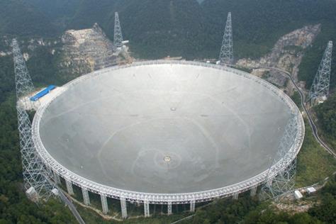
Figure: The 500-metre Aperture Spherical Telescope (FAST) at Guizhou, China [South China Morning Post].

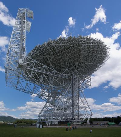
Figure: 100-m diameter 0.1-116 GHz fully steerable radio telescope antenna in Green Bank, West Virginia, US [Wikipedia].

Figure: A 26-m prime-focus parabolic reflector antnena and a 12-m AuScope VLBI antenna at the Mount Pleasant Radio Observatory (Australia) [Wikipedia].

Figure: High-performance backfire feed [From Garcia-Perez].

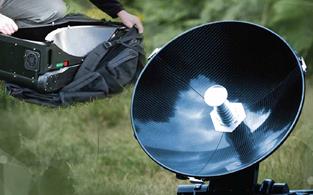
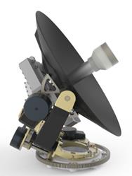
Figure: Left = General Dynamics uPak C060QDA 60-cm reflector antenna for SATCOM on the move (SOTM) operating at Ka, Ku, and X bands. Right = Skytech 30-cm ADE reflector for SOTM (Rx 10.7-12.75 GHz, Tx 13.75-14.5 GHz)

Figure: Gain patterns of a 10.3-λ backfire fed parabolic reflector antenna. From Kildal, IEEE T-AP, 45(7), 1997

References

[1] T. A. Milligan, Modern Antenna Design, 2nd Edition, IEEE-Wiley, 2005.

[2] W. L. Stutzman and G. A. Theiele, Antenna Theory and Design, 3rd Edition, Wiley, 2013