실습 04 – 반파장 다이폴
1. 이론
ㅇ 반파장 다이폴은 길이가 0.35-0.48파장(다이폴 단면에 따라 변함)인 금속의 중간에서 급전하는 안테나이다.
ㅇ 가장 기본적인 안테나로서 기본형과 응용구조가 널리 사용된다.
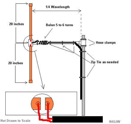
<FM 방송 송신안테나>
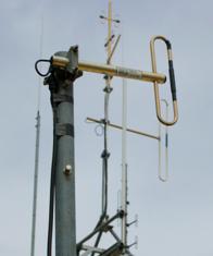
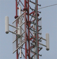
<무선통신 안테나>
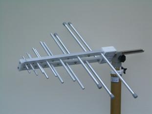
<EMC 시험용 광대역 대수주기 다이폴>
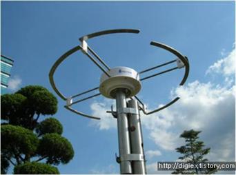
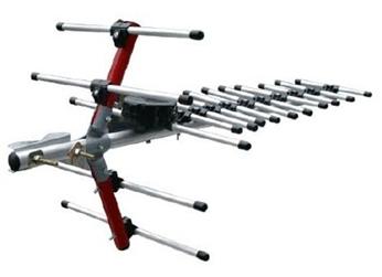
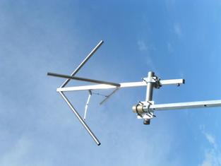
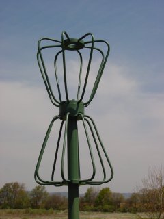
<DTV 수신용 무지향성 안테나> <DTV 수신용 고이득 야기 안테나>
ㅇ 다이폴 설계 시 핵심은 대역폭, 급전, 다이폴의 크기이다.
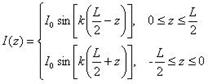
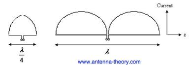
ㅇ 다이폴의 전류분포: 중심을 기준으로 대칭적 정현파 분포
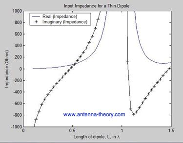
ㅇ 다이폴의 입력 임피던스: 임피던스는 주파수에 따라 변하며 허수부가 0이 되는 최초 공진은 다이폴 길이가 반파장 부근일 때 발생. 이 때 입력 저항은 약 72W
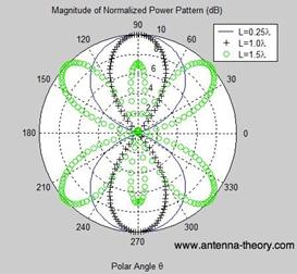
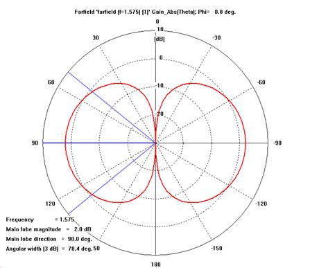
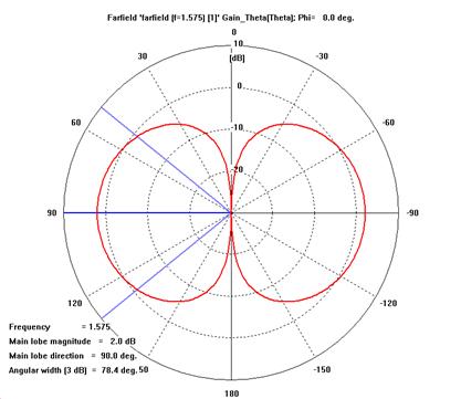
ㅇ 다이폴의 방사패턴: 3dB 빔폭 78°
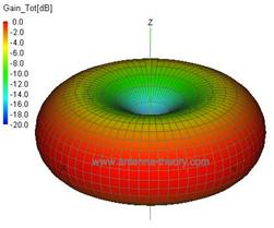
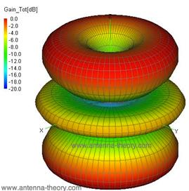
ㅇ 다이폴의 이득(지향도)
– 길이가 매우 작을 때: D
= 1.50 = 1.76 dBi
– 반파장 다이폴: D
= 1.64 = 2.15 dBi
ㅇ 상용제품 예:
2) Dipole
- A dipole is a two-piece straight metal antenna fed at the center.
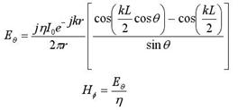
- When a half-wave dipole is placed along the z-axis, at far fields we have ![]() .
.
- The radiation pattern of a half-wave dipole resembles the number 8 with a maximum occurs in the direction normal to the dipole axis while a null occurs in the direction of the dipole axis.
- Half-wave beamwidth and gain of a half-wave dipole are 78º and 2.1dB respectively.
Fig. 5.4 A dipole and its radiation pattern.
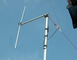
Fig. 5.5 A 2-m dipole antenna.
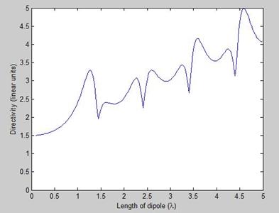
- The dipole's impedance changes with the frequency. Its first resonance is at the frequency where its total length is about a half wavelength (to be more exact, L = 0.468λ). At resonance the dipole's input impeance is about 70+j0 (Ω).
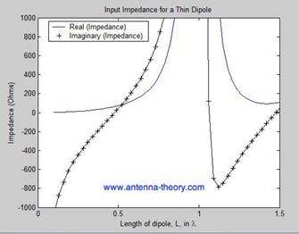
Fig. 5.6 The dipole input impedance versus the length.
- A dipole is often fed by a coaxial cable. In this case there is an imbalance in the magnitude of currents on two halves. Even with this current imbalance, one can still use a coaxial cable feeding for the sake of simplicity.
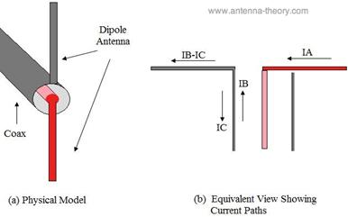
Fig. 5.6 A coax-fed dipole and the current
imbalance.
2. 실습
1) Draw
the geometry.
- Draw
the following geometry of a dipole with dimensions:
d = 0.5mm (You will fabricate the dipole using a thin wire used
for wiring components on the breadboard)
L = λ/2 @ 1.575GHz
= 95.2mm
g = 0.1
mm
- Be
sure to make the dipole axis be in the z
direction. In this case, the E-plane
is zx- or yz-plane
and the H-plane is the xy-plane.

2)
Simulate and tune the antenna.
- Use a
discrete port (a delta-gap source) for the excitation.
-
Frequency range: 0.2 to 3.2GHz.
- With
the initial dimension, your antenna will resonate at 1.46GHz.
Using the following formula based on
the theory of frequency scaling, we find the dipole length
for a resonance at 1.575GHz.
![]()
![]()
- Now
adjust the dipole length to 88.2mm and do the
simulation again.
3)
Analyze the result and write a report.
-
Analyze the result, that is, see simulation results and form your opinions on
them.
- In
making graphs, make sure that sizes of axis labels, scale values are big
enough.
○ Near field at 1.575GHz:
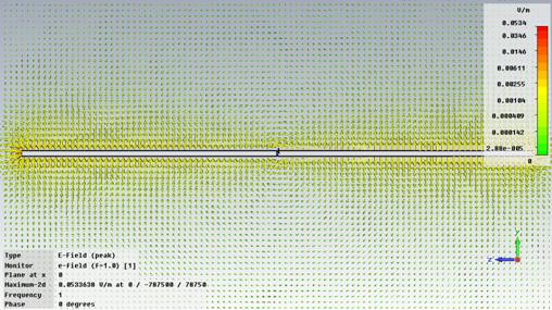
- Observe the electric field around the
dipole using stationary and animated views.
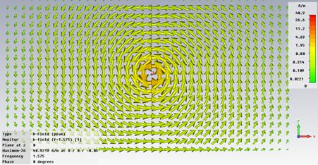
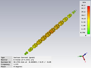
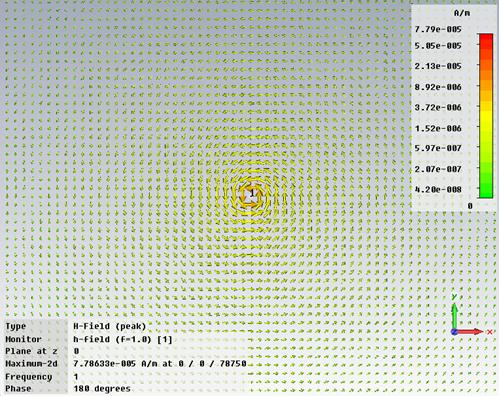
- Observe the magnetic field (or the
equivalent electric current) around the dipole. The surface electric current
density on a conductor is related to the magnetic field
![]()
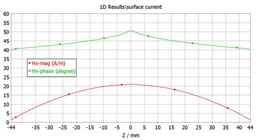
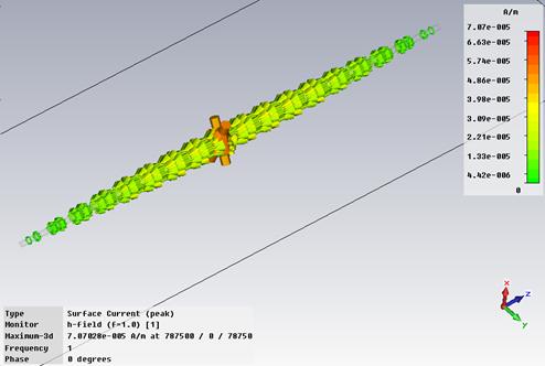
- Plot the magnitude and phase of Jz
along the surface of the dipole on the same graph.
○ Input
impedance:
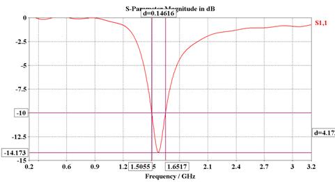
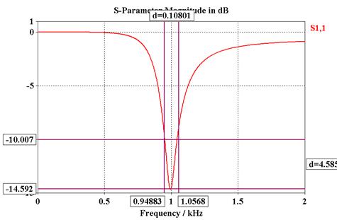
- |S11|(dB)
from 0.2 to 3.2GHz. Find the impedance bandwidth (|S11|
< -10dB) with two vertical cursors.
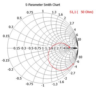
- Plot the impedance locus on the Smith
chart from 1.0 to 2.0GHz.
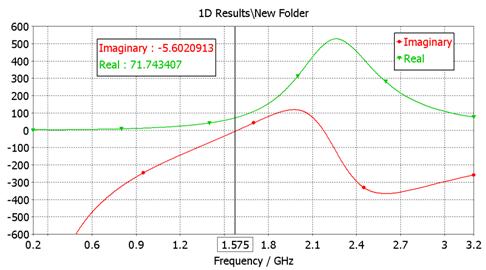
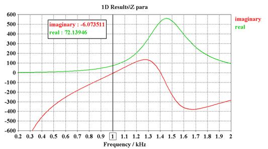
- Plot Rin and Xin
from 0.2 to 3.2GHz on the same graph. Mark Rin
and Xin
at 1.575GHz with a vertical cursor.
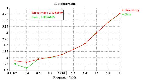
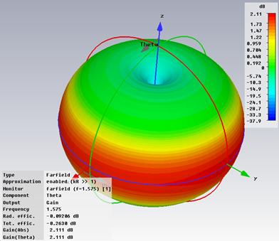
○ Gain
and directivity:
- G(dB) and D(dB)
from 0.2 to 3.2GHz by 0.2GHz
step on the same plot.
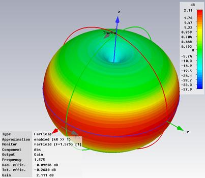
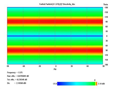
○ Gain
pattern at 1.575GHz:
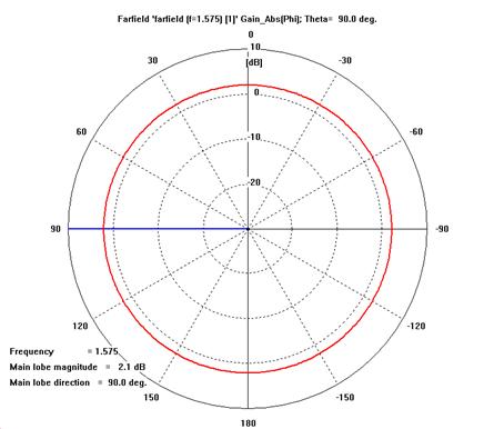
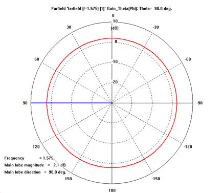
- Gabs:
3D, E-plane
polar pattern, H-plane polar pattern
- Gθ: 3D, E-plane polar
pattern, H-plane polar. Mark the 3dB beamwidth on the polar plot.
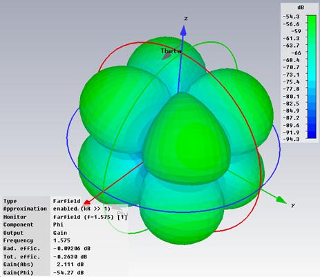
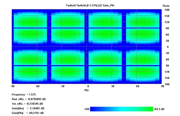
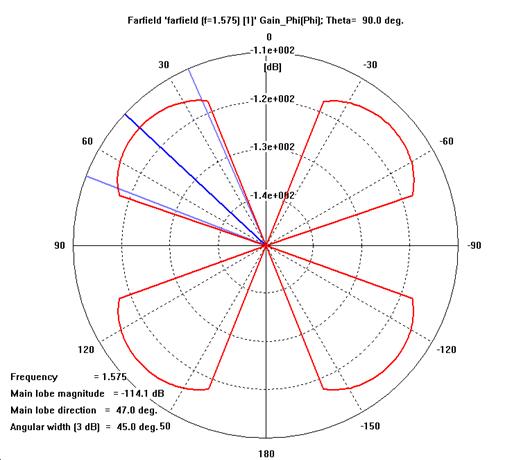
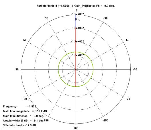
- Gφ: 3D, E-plane polar
pattern, H-plane polar pattern
- Write
a full report using graphs from the simulation software.
- Give
the antenna geometry, dimensions and the method of excitation. Include the
coordinate axis.
-
Present graphs described in the above and give your assessment of the results.
- Make a
hand-written report on the spot as follows.
- Describe the antenna geometry,
dimensions and the feeding method. Include the coordinate axis.
- Plot the magnitude of Jz
along the surface of the dipole. Give your analysis of the result.
- Input impedance:
- |S11|(dB)
= ( ) @ 1.575GHz
- Impedance bandwidth (-10dB reflection)
- Zin = ( ) + j( ) ohms @ 0.2, 1.0,
1.575, and 2.0GHz
- Gain and directivity:
- Gθ(dB) = ( ) @ 0.2, 1.0, 1.575, 2.0GHz. Give your analysis of the result.
- Dθ(dB) = ( ) @ 0.2, 1.0, 1.575, 2.0GHz. Give your analysis of the result.
- Gain patterns at 1.575GHz:
- Plot Gθ(dB), Gφ(dB)
on E-plane. Give your analysis.
- Plot Gθ(dB), Gφ(dB)
on H-plane. Give your analysis.
- E-plane
beamwidth = ( )
deg.
4)
Simulation results.
-
Electric field E around the dipole
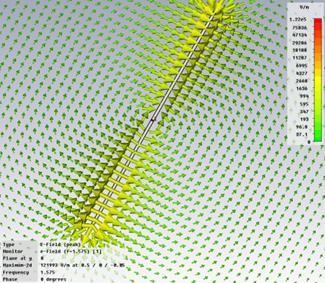
-
Magnetic field H around the dipole
-
Current density J on the dipole
surface
-
Magnitude and phase of Jz
along the surface of the dipole
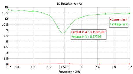
(Question) In a discrete
port, what is the terminal voltage or current?
- Terminal voltage and current of the discrete port vs frequency
- Reflection coefficient: bandwidth = 146.2MHz
(9.3%)
- Input
impedance locus on the Smith chart
- Input impedance ![]() . Inaccurate results below 1GHz.
Why is the accuracy below 1GHz poor? We have to
increase the accuracy setting in the 'Solve' - 'Transient Solver Parameters' menu.
Increase the accuracy from -30dB to -60dB for example.
. Inaccurate results below 1GHz.
Why is the accuracy below 1GHz poor? We have to
increase the accuracy setting in the 'Solve' - 'Transient Solver Parameters' menu.
Increase the accuracy from -30dB to -60dB for example.
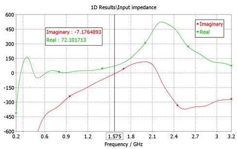
- Input impedance ![]() . Accurate results.
. Accurate results.
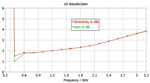
- Gain
and directivity. vs frequency. Inaccurate below 1GHz.(MWS
Transient Solver accuracy setting: -30dB)
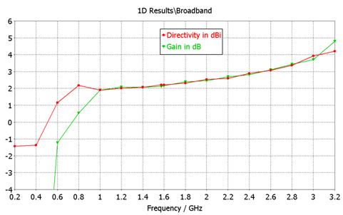
- Gain
and directivity. vs frequency. Inaccurate below 0.4GHz.(MWS
Transient Solver accuracy setting: -60dB)
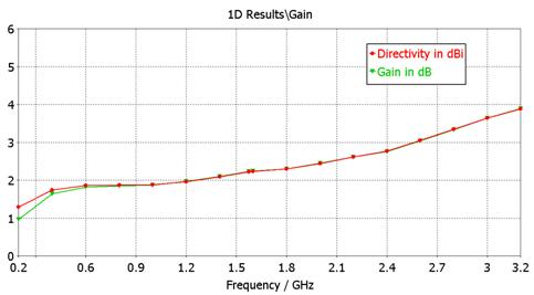
- Gain and
directivity. vs frequency. Accurate
results. (MWS Transient Solver accuracy
setting: -60dB). The
absorbing boundary is too close to the antenna. We have to increase the
distance from the dipole to the absorbing surfaces of the rectangular box enclosing
the dipole.
(Supplementary Simulations)
Dipole resonating at 1kHz: L = 138,915m (0.463![]() ), d = 788m, g = 176m
), d = 788m, g = 176m
- Electric field E
around the dipole
-
Magnetic field H around the dipole
-
Current density J on the dipole
surface
- Reflection coefficient: bandwidth = 108Hz
(10.8%)
- Input
impedance locus on the Smith chart
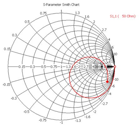
- Input impedance ![]() .
.
- Gain
and directivity. vs frequency.
- Gabs
- Gθ

- ![]()