Radio Frequency Systems Engineering (고주파시스템공학)

1. 공지사항

ㅇ Grading: 출석 10%, 과제 15%, 실습 15% 중간시험 30%, 기말시험 30%

ㅇ Textbook:

- 원서: D. M. Pozar, Microwave Engineering, 4th Ed., Wiley, 2015.

- 번역서: 마이크로파공학 (D. M. Pozar 저), 고지환 역, 한티에듀, 2020.

ㅇ 과제용 학생고유번호 PIN: 학교에 등록된 자신의 이동전화 끝 4자리. 단 각 숫자가 0인 경우 순차적으로 1, 2, 3, 4로 대체. 예시: 4321 → 4321, 4010 → 4112

ㅇ 과제 제출: eCampus에 업로드. 다음 주 수업일 23:59까지. 수기답안 촬영하여 업로드

ㅇ 실습결과 제출: SW중심대학 코딩이력관리시스템에 업로드

ㅇ 강의관련 문의사항: 담당교수 bician@cbu.ac.kr (E10-611)

조교: 허지원 gjwldnjs131@naver.com (E10-519)

ㅇ SW 중심대학 사업단 코딩이력관리 시스템: https://sw7up.cbnu.ac.kr/project/dashboard 접속하여 업로드. 사용설명서 ; 파일명을 *.c, *.py, *.cpp 으로 업로드

2. 주별 강의

3학년 학생을 위한 조언

Week-01: Intro to RF Systems

Lecture (pdf)

(과제) 자기분석; 정해진 양식 없음. ® eCampus에 업로드

문제1=1.1-2.2 학기 되돌아 보기

문제2=3.1-4.2학기 학업/역량향상 계획수립

문제3=졸업후 진로/취업계획

Week-02: Transmission Lines 1

이론강의: 5G Smartphone RF Front End Technology (pdf)

이론강의 (pdf, pptx-no-voice, pptx-voice, mp4)

실습강의 (pdf, htm), 음성강의(파이썬사용법&실습3번, 실습1번&2번, 실습4번)

학생실습 (pdf, htm): 수업시간 내에 코딩이력관리시스템에 업로드한 후에 조교 채점

이론숙제: 다음 수업일까지 eCampus 업로드

1. Express the characteristic impedance Z₀ of a transmission line in terms of R, L, G, and C.

2. Express the complex propagation constant γ of a transmission line in terms of R, L, G, and C.

3. Express Z₀ and γ of a lossless transmission line in terms of L and C.

4. Write down a Python program and execute it to find the characteristic impedance Z₀ and the complex propagation constant γ of a transmission line with R = 176 mΩ/m, L = 490 nH/m, G = 2 μS/m, C = 49 pF/m. Accept the frequency f while the code runs as an input data of your choice.

Week-03: Transmission Lines 2

이론강의: AI on Mobile Devices (pdf)

이론강의 (pdf, pptx-no-voce, pptx-voice, mp4)

실습강의 (pdf, htm), 음성강의(mp4)

학생실습 (pdf, htm): 수업시간 내에 코딩이력관리시스템에 업로드한 후에 조교 채점

(참고) 과제문제 풀때 필요하면 다음의 복소수 계산기 사용

복소수 계산기: 직각좌표/극좌표 형식 변환, 곱셈, 뺄셈

Python: complex_calc_1_python.txt

Fortran: complex_calc_1.f90, complex_calc_1.exe

이론숙제: 다음 수업일까지 eCampus 업로드

PIN=pqrs, a = p+q+r+s, b = 3*a

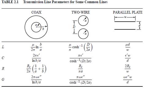
Coaxial cable with a(given above), b(given above), μ_r = 1, ε_r = 2, tanδ = 0.001, σ = 5.8e7 S/m, f = 5.8 GHz

Calculate Z₀, γ, R, L, G, C, α_c (dB/m), α_d (dB/m), α (dB/m), λ_g.

(참고) 다음 공식 사용

Week-04: Transmission Lines 3

이론강의: Review of the AI Chatbot (pdf)

이론강의 (pdf, pptx-no-voice, pptx-voice, mp4)

실습강의 (pdf, htm), 음성강의(mp4)

학생실습 (pdf, htm): 수업시간 내에 코딩이력관리시스템에 업로드한 후에 조교 채점

이론숙제: 다음 수업일까지 eCampus 업로드

Visit http://mcalc.sourceforge.net/ to analyze a microstrip line.

다음과 같이 설정

단위를 mm 설정

Er = 4.3, Rho =1

H = 1, Rough = 0.0

Tmet = 0.035, Tanδ = 0.02

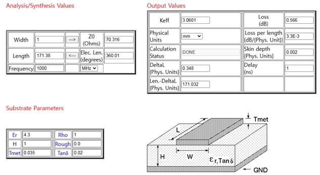
Keff는 ε_re (유효 유전상수)

선로파장:

Elec. Len. (degrees) = 선로의 전기적 길이를 각도로 표현. 1파장은 360°에 대응된다.

(문제)

W = 2mm, Frequency = 1500MHz 인 경우 Z0, Keff, L (1파장의 길이)를 구하라. 이 경우 Loss (dB)를 구하라.

Week-05: Smith Chart

이론강의: AI Tools (pdf)

이론강의 (pdf, pptx-no-voice, pptx-voice, mp4)

실습강의 (pdf, htm, mp4)

학생실습 (pdf, htm): 수업시간 내에 코딩이력관리시스템에 업로드한 후에 조교 채점

이론숙제: 다음 수업일까지 eCampus 업로드

PIN=abcd (PIN=3194, a=3, b=1, c=9, d=4)

1. Draw a r = a circle on a Smith chart.

2. Draw a x = d circle on a Smith chart.

참고:

스미스도표 양식: Smith-z-chart, Smith-y-chart, Smith-zy-chart

Python에서 복소수 계산

Wee-06: Impedance Matching 1

기말시험: 8주차 수업시간, 오픈북, 스마트폰/태블릿/컴퓨터 미사용, 50분간, 코딩문제포함

유용한 교양강좌(htm)

이론강의 (pdf, pptx-no-voice, pptx-voice, mp4)

실습강의자료 (pdf, htm), 음성강의 (mp4)

학생실습 (pdf, htm): 수업시간 내에 코딩이력관리시스템에 업로드한 후에 조교 채점

이론숙제: PIN=abcd (example: PIN=3194, a=3, b=1, c=9, d=4)

Vs = 10a × exp(j20°)

Zs = 10b + j 10c (ohm) : connected in series with Vs

ZL = 30a − j 40d (ohm) : connected in series with Zs

1. Find the power PL (W) at ZL

2. Modify ZL for maximum power transfer.

3. Find the power PL (W) at ZL when ZL is modified for the maximum power transfer.

Week-07: Impedance Matching 2

이론강의 (pdf, pptx-no-voice, pptx-voice, mp4)

실습강의 (pdf, htm), 음성강의(mp4)

학생실습 (pdf, htm): 수업시간 내에 코딩이력관리시스템에 업로드한 후에 조교 채점

(참고) LC matching: Python souce code (python-general LC matching.doc)

이론숙제: 다음 수업일까지 eCampus 업로드

PIN=abcd (example: PIN=3194, a=3, b=1, c=9, d=4)

1. Find all the possible element values of LC-matching networks that transforms 10a+j40b Ω to 50 Ω. Use the Python code given above.

Week-08: Mid-term Exam

중간고사: 문제(doc), 시험시간 50분, 수기답안 제출, 오픈북(강의노트, 공부노트, 책 등), 정보기기(스마트폰 등) 미사용

Week-09: Passive RLC Components 1 - Resistors

이론강의 (pdf, pptx-no-voice, pptx-voice, mp4) (음성강의자료는 작업중이며 금일중 업로드됩니다.)

실습강의 (pdf, htm), 음성강의(mp4)

학생실습 (pdf, htm): 수업시간 내에 코딩이력관리시스템에 업로드한 후에 조교 채점

이론숙제: 다음 수업일까지 eCampus 업로드

PIN=abcd (example: PIN=3194, a=3, b=1, c=9, d=4)

1. Resistor equivalent circuit

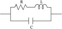
1) Find an expression for the impedance.

2) f = a MHz, R = 100b (ohm), L = b nH, C= 2d pF. Calculate the impedance.

Week-10: Passive RLC Components 2 - Capacitors

이론강의 (pdf, pptx-no-voice, pptx-voice, mp4)

실습강의 (pdf, htm), 음성강의(mp4)

학생실습 (pdf, htm): 수업시간 내에 코딩이력관리시스템에 업로드한 후에 조교 채점

이론숙제: 다음 수업일까지 eCampus 업로드

PIN=abcd (example: PIN=3194, a=3, b=1, c=9, d=4)

1. Capacitor equivalent circuit

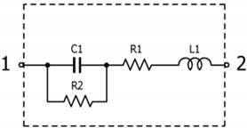
1) Find and expression for the impedance.

2) f = 100a MHz, C1 = 20b nF, R2=b Gohm, R1=c/100 ohm, L1 = d/4 nH. Calculate the impedance.

Week-11: Passive RLC Components 3 - Inductors

이론강의 (pdf, pptx-no-voice, pptx-voice, mp4)

실습강의 (pdf, htm), 음성강의(mp4)

학생실습 (pdf, htm): 수업시간 내에 코딩이력관리시스템에 업로드한 후에 조교 채점

이론숙제: 다음 수업일까지 eCampus 업로드

PIN=abcd (example: PIN=3194, a=3, b=1, c=9, d=4)

1. Inductor equivalent circuit

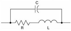
1) Find and expression for the impedance.

2) f = 100a MHz, R=10b ohm, L = 5b μH, C = d/10 pF. Calculate the impedance.

Week-12: Maxwell's Equations and Wave Equation

이론강의 (pdf, pptx-no-voice, pptx-voice, mp4)

실습강의 (pdf, htm), 음성강의(mp4)

학생실습 (pdf, htm): 수업시간 내에 코딩이력관리시스템에 업로드한 후에 조교 채점

이론숙제: 다음 수업일까지 eCampus 업로드

PIN=abcd (example: PIN=3194, a=3, b=1, c=9, d=4)

1. f = 1 GHz, εr = a, μr = b. Find the wavelength and the intrinsic impedance.

Week-13: Communication Systems and Link Budget

이론강의 (pdf)

강의노트 문제 코딩 = Take-Home Final Exam. (13주 과제란에 제출: 마감 6월14일23:59)

PBL (Project-Based Learning) Lecture 1 (pdf)

PBL 팀원(A,B,C) 업무분담:

보고서: 요약=A, 1. 서론=B, 2. 이론=C, 3. 실험=A,B,C(각자 코딩; 실행; 각자 3.실험 작성하여 취합(각자 작성한 부분 그대로 수록), 결론=A,B,C(각자 결론 작성하여 취합; 각자 작성한 부분 그대로 수록)

이론숙제: 다음 주 수업일까지 eCampus 업로드

Make a Python code. Include the result of code execution.

Receiver thermal noise

(Input)

ts: receiver noise temperature (K)

b: receiver bandwidth (Hz)

(Output)

n: receiver thermal noise power (W)

ndBm: receiver noise power in dBm

Week-14: Radar Systems and Radar Equation

이론강의 (pdf)

강의노트 문제 코딩 = Take-Home Final Exam. (14주 과제란에 제출)

PBL Lecture 2 (pdf)

이론숙제: 없음.

Week-15: Final exam.

기말시험은 PBL 보고서로 대체합니다: 희망팀은 강의시간에 학교에서 와서 조교와 담당교수의 도움을 받을 수 있음.

PBL 보고서 = 15주차 과제란에 제출 (마감 6월14일23:59)